Review: Fast-SCNN
In this post, Fast-SCNN (fast segmentation convolutional neural network) [1] is briefly reviewed. This architecture aims on real-time semantic segmentation tasks, and it can reach 123.5 frames per second on Cityscapes dataset with a high resolution of input image (1024 x 2048 px), while with small capacity network size.
Outline
- Fast-SCNN Architecture
- Learning to Downsample
- Experiment Results
- Ablation Studies
1. Fast-SCNN Architecture
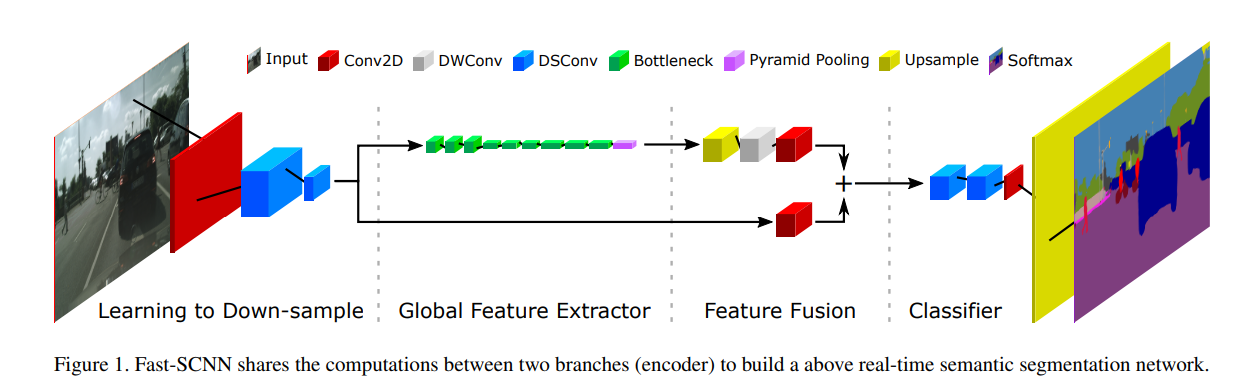
- As shown above, Fast-SCNN is composed of four modules: Learning to Downsample, Global Feature Extractor, Feature Fusion, and Classifier.
- All modules are built using depth-wise separable convolution.
- The reason is that such convolution has become a key building block adopted by many efficient
DCNN architectures such as Xception, MobileNet, and Contextnet.
- The reason is that such convolution has become a key building block adopted by many efficient
DCNN architectures such as Xception, MobileNet, and Contextnet.
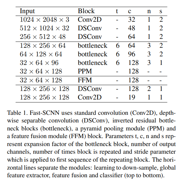
- The layout is shown above, where the horizontal lines separate the modules.
- Parameter explanation
- t: expansion factor of the bottleneck block
- c: number of output channels
- n: number of times that block is repeated
- s: stride parameter which is applied to first sequence of the repeating block
- Parameter explanation
2. Learning to Downsample
- Current state-of-the-art real-time semantic segmentaiton methods are built by networks with two
braches operating on distinct resolutions on each side.
- The methods learn global information from low-resolution versions of the input image, and shallow networks refine the precision of the segmentation results on full input resolution.
- As the well-known fact that DCNNs extract the low-level features such as corners and edges on the first few layers, the authors think that sharing feature computation between the low and high -level branch in a shallow network block will boost up the performance.
3. Experiment Results
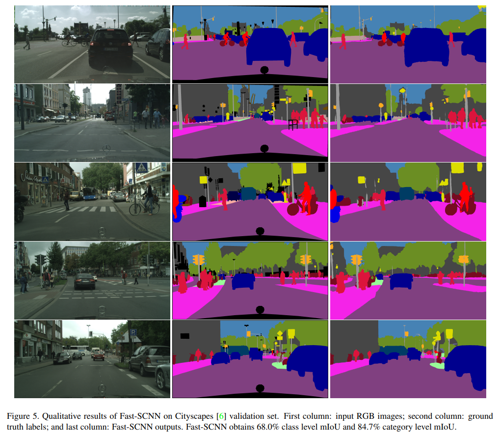
- The authors evaluate Fast-SCNN on Cityscapes dataset.
- Furthermore, they add 20,000 weakly annotated images, or coarse labels, on training.
- They report results with three groups: both, fine only, and fine with coarse labeled data.
- They Use only 19 classes on evaluation.
- As comparison, ContextNet, BiSeNet, GUN, ENet, and ICNet are chosen as they are SOTA real-time semantic segmentation methods.
- The proposed Fast-SCNN is divided to two types: Fast-SCNN cls and Fast-SCNN prob on the part
of runtime comparison.
- The reason of doing this is that softmax operation is costly on inferencing; as a consequence, they replace softmax to argmax when the network is on inference mode.
- Fast-SCNN cls denotes the softmax is changed to argmax.
- Fast-SCNN prob denotes the standard version.
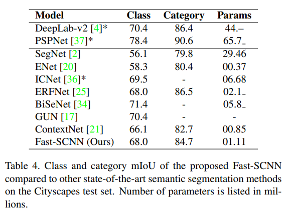
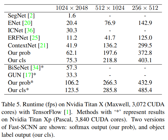
- The above tables shows Fast-SCNN outperforms other STOA methods.
4. Ablation Studies
Pre-training and Weakly Labeled Data
- High capacity DCNNs such as R-CNN and PSPNet have shown that performance can be boosted with pre-training through contrast auxiliary missions.
- As the authors specify Fast-SCNN having low capacity, they want to test performance with
and withoug pre-training, and with the connection with and without additional weakly
labeled data.
- Also, it seems that the importance of pre-training and additional weakly labeled data on DCNNs with low capacity has not been studied before.
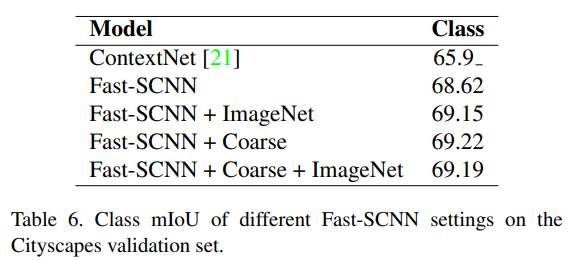
- As shown in Table 6, it seems neither pre-training nor weakly labeled data boosts up the performance for low capacity DCNN.
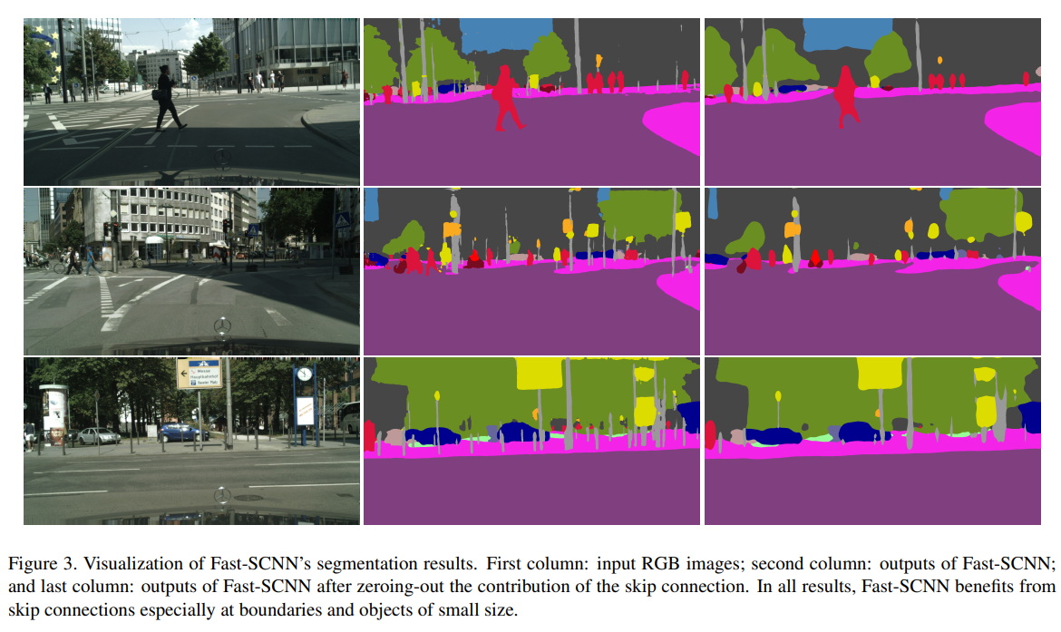
Zero-out Skip Connection
- The authors make this test to confirm whether skip connection benefits Fast-SCNN or not.
- By zeroing-out skip connection, the mIoU drops from 69.22% to 64.30% on the validation
dataset, and Figure 3 shows the results between without and with zeroing-out skip
connection.
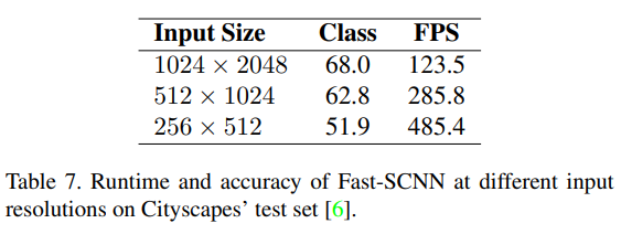
Lower Input Solutions
- Since the authors are having interests on those embedding devices without full resolution input or powerful computational power, they study this with half and quarter input resolutions.
- Shown in Table 7, the authors conclude Fast-SCNN is directly applicable to lower input
resolution without modification.
Reference
[1] https://arxiv.org/abs/1902.04502